Diffusion Models: A New Playground for Reinforcement Learning

Reinforcement learning (RL) has achieved remarkable progress in solving complex decision-making problems, from playing Go and mastering Atari games (Schrittwieser et al., 2019) to robotic control. Yet, one major limitation remains — sample inefficiency. RL agents often require millions of interactions with their environments to learn effective policies. In the real world, such exhaustive trial-and-error is often impractical or prohibitively time expensive.

To address this, researchers have turned to world models — generative models that learn to simulate environments. Instead of interacting with the real world at every step, an agent can learn by imagining outcomes within its learned world model. This idea, popularized by works like World Models (Ha & Jü, 2018), has inspired a line of research into using generative modeling as a core component to train RL agents.

Figure 1: A World Model. Credit to (Scott McCloud, 1993) .

Over time, a variety of generative modelling approaches have been explored to serve as effective world models, including Variational Autoencoders (VAEs), Generative Adversarial Networks (GANs), and Flow-based models.

• VAEs are stable and easy to train but rely on a surrogate loss, which can lead to blurry reconstructions (Kingma & Welling, 2013). This can be limiting when high-fidelity state predictions are required for planning in RL.
• GANs can produce highly realistic samples, but their adversarial training often leads to instability and mode collapse, resulting in limited diversity — a critical drawback when trying to capture all possible environment states (Goodfellow et al., 2014) (Martí, 2017) .
• Flow-based models learn bijective mappings between data and latent spaces, allowing for exact likelihood estimation and stable training (Rezende & Mohamed, 2015). However, they require carefully designed architectures to maintain reversibility, which can limit flexibility and scalability in modeling complex, high-dimensional environments.

While VAEs, GANs, and flow models have all been explored as world models, each involves trade-offs that can affect their use in RL. This has led researchers to investigate diffusion models, a newer class of generative models with a different approach to modeling data distributions.

The Basics of Diffusion Models

Diffusion models are inspired by non-equilibrium thermodynamics, where systems naturally evolve from low-entropy (ordered) states to high-entropy (disordered) states. They define a Markov chain of diffusion steps that gradually add random noise to data, mimicking the physical process of diffusion. The model then learns to reverse this process — transforming noise back into structured data — effectively moving from a high-entropy to a low-entropy state.

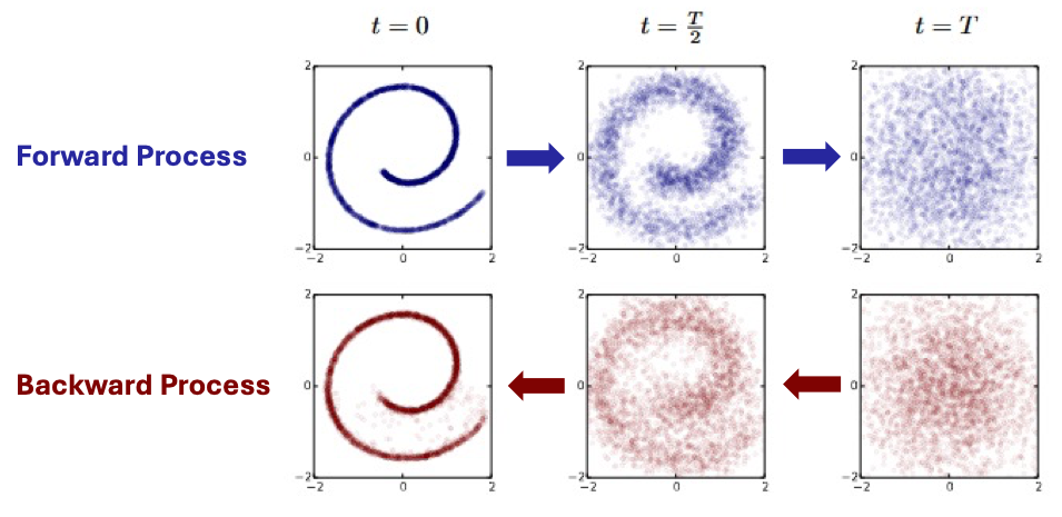
Figure 2: Example of a trained diffusion model for modeling a 2D swiss roll data. Credit to (Sohl-Dickstein et al., 2015) .

Through this learned denoising dynamics, diffusion models can generate realistic data samples by starting from random noise and iteratively reconstructing the underlying structure of the data distribution. Conceptually, this can be seen as an encoding–decoding process, like VAEs or flow-based models, where the forward diffusion “encodes” data into a noisy latent and the reverse process “decodes” it back into structured samples. However, unlike VAEs or flows, the forward procedure is fixed (not learned), and the latent variables have the same dimensionality as the original data rather than being compressed into a smaller latent space.

The forward and backward processes in diffusion models can be formulated in both discrete and continuous forms. We will briefly mention the discrete form as it is the original historical formulation, but our focus will be on the continuous form, which is more generic and better captures complex, high-dimensional dynamics.

In the discrete-time formulation, the forward process gradually adds noise to a data sample $x^0$ over $T$ timesteps, producing a sequence ${x^1, x^2, \dots, x^T}$. At each step $\tau$, noise is added according to a predefined schedule $\beta_\tau$:

\[x^\tau = \sqrt{1 - \beta_\tau} \, x^{\tau-1} + \sqrt{\beta_\tau} \, \epsilon_\tau, \quad \epsilon_\tau \sim \mathcal{N}(0, I)\]

The backward process learns to reverse this noising process by estimating the conditional distribution $p_\theta(x^{\tau-1} \mid x^\tau)$, typically parameterized by a neural network.

In the continuous-time formulation, the forward process is modeled as a stochastic differential equation (SDE), which smoothly diffuses the data into noise:

\[dx = f(x, \tau) \, d\tau + g(\tau) \, dW_\tau\]

where $f(x, \tau)$ represents a predefined deterministic drift term, $g(\tau)$ a predefined diffusion coefficient, and $dW_\tau$ denotes a Wiener process (Brownian motion).

The backward process then corresponds to a reverse-time SDE, which removes noise by following the time-reversed dynamics:

\[dx = [f(x, \tau) - g(\tau)^2 \nabla_x \log p_\tau(x)] \, d\tau + g(\tau) \, d\bar{W}_\tau\]

where $d\bar{W}_{\tau}$ represents the reverse-time Wiener process and $\nabla_x \log p_\tau(x)$ the score function of the noisy distribution at time $\tau$.

The score function $\nabla_x \log p_\tau(x)$ represents the gradient of the log-probability of the data at time $\tau$, pointing toward regions of higher likelihood. It adjusts the drift $f(x, \tau)$ in the reverse-time SDE, guiding $x$ to produce realistic samples.

Since the distribution $p_\tau(x)$ is generally unknown, the score function $\nabla_x \log p_\tau(x)$ is also unknown and must be estimated from data. Diffusion models achieve this by leveraging a combination of sampling and learning. A typical approach assumes that the deterministic shift function $f(x, \tau)$ is affine, which simplifies the mathematics and allows the forward diffusion process to reach any intermediate time $\tau$ analytically using a Gaussian perturbation kernel $p^{0}_ {\tau}(x^\tau \mid x^0)$. The procedure then proceeds as follows:

1. Sample clean data $x^0$ from the target distribution.
2. Corrupt the samples by simulating the forward diffusion to obtain $x^\tau$ at the desired time $\tau$. If $f$ is affine, this can be done in a single step using the known Gaussian kernel.

3. Train a score model $s_\theta(x, \tau)$ to estimate the score function by minimizing a denoising objective such as (Karras et al., 2022):

   \[\mathbb{E}_{x^0, x^\tau \sim p^{0}_{\tau}} \left[ \left\| s_\theta(x^\tau, \tau) - \nabla_{x^\tau} \log p^{0} _{\tau}(x^\tau \mid x^0) \right\|^2 \right]\]

Once trained, this score model provides an approximation of $\nabla_x \log p_\tau(x)$ at any time $\tau$, allowing the backward SDE to iteratively denoise samples and generate realistic data from pure noise.

Diffusion Models for World Modelling

In the context of world modeling for sequential decision-making, the goal is to learn a generative model of the environment dynamics — that is, to predict the next observation of the system given past observations and actions. Formally, we aim to model a conditional generative distribution: \(p_\theta(x_{t+1} \mid x_{\le t}, a_{\le t}),\)

where $x_{t+1}$ is the next (unknown) observation, $x_{\le t} = {x_0, \dots, x_t}$ are past observations, and $a_{\le t} = {a_0, \dots, a_t}$ are past actions. Unlike unconditional diffusion models, here the diffusion model must condition on the history of observations and actions to accurately predict the future.

To train a diffusion model for world modeling, we first need to collect trajectories $(x_0, a_0, x_1, a_1, \dots, x_t, a_t, x_{t+1})$ from the real environment to obtain clean next observations $x_{t+1}$ as targets. Once we have these trajectories, we treat $x_{t+1}$ as the “clean” data and corrupt it with a Gaussian perturbation kernel to produce a noisy sample $x_{t+1}^\tau$. The model then learns a conditional score function $s_\theta(x_{t+1}^\tau, \tau \mid x_{\le t}, a_{\le t})$ that estimates the gradient of the log-probability of the noisy next observation. The training objective is the following loss:

\[\mathcal{L}(\theta) = \mathbb{E}_{x_{t+1}, \, x_{t+1}^\tau \sim p^0_\tau} \Big[ \| s_\theta(x_{t+1}^\tau, \tau \mid x_{\le t}, a_{\le t}) - \nabla_{x_{t+1}^\tau} \log p^0_\tau(x_{t+1}^\tau \mid x_{t+1}) \|^2 \Big],\]

which encourages the model to reverse the corruption process and recover $x_{t+1}$ conditioned on past observations and actions.

Once the diffusion model is trained, it can be used as a generative model for decision-making. In this setting, the next observation $x_{t+1}$ is typically unknown and is initially represented either as Gaussian noise or a prior estimate. The model then iteratively denoises this sample, step by step, using the reverse-time SDE, conditioned on past observations and actions. This procedure generates a realistic prediction of the next state, which can be used to train a RL agent.

Figure 3: The diffusion model takes into account the agent's action and the previous frames to simulate the environment response. Credit to (Alonso et al., 2024).

Iterative Training of the Reinforcement Learning Agent and the Diffusion Model

In general, diffusion models and reinforcement learning (RL) agents are not trained fully separately but rather in an iterative loop, where both models are improved in alternating phases. The typical procedure involves three main steps:

1. Collect real data: The RL agent interacts with the real environment collecting trajectories of observations, actions,rewards, and termination signals in a replay buffer.

2. Train the world model: A diffusion-based world model is trained using all data from the replay buffer. In addition to modeling the next observation, auxiliary components such as a reward model and a termination model are included to fully capture the environment dynamics.

3. Train the RL agent in imagination: Once the world model is trained, it replaces the real environment during policy optimization. The agent is trained by imagining trajectories—simulating rollouts within the learned model—using the predicted next observations, rewards, and terminations.

These three steps are repeated in a loop, allowing the world model to continuously refine its understanding of the environment while the RL agent progressively improves its policy through imagined experiences.

A Promising Example

A recent paper, Diffusion for World Modeling: Visual Details Matter in Atari (Alonso et al., 2024), presents DIAMOND, a RL-agent trained on a diffusion-based world model that achieves impressive performance on the Atari 100k benchmark. This benchmark evaluates agents across 26 Atari games, where each agent is allowed only 100k real environment interactions—roughly equivalent to two hours of human gameplay—to train its world model. For context, traditional RL agents without world models are typically trained in the environment for up to 50 million steps, meaning DIAMOND needs 500× less interactions with the environment.

DIAMOND is compared against several state-of-the-art world model agents, including STORM (Zhang et al., 2023), DreamerV3 (Hafner et al., 2023), IRIS (Micheli et al., 2023), TWM (Robine et al., 2023), and SimPle (Kaiser et al., 2019). In aggregate performance, DIAMOND achieves a superhuman mean human-normalized score (HNS) of 1.46, outperforming all previous world model agents, and exceeding human-level performance on 11 out of 26 games. Notably, its interquartile mean (IQM) performance matches that of STORM while surpassing all other baselines, demonstrating consistent performance across games. DIAMOND particularly excels in visually detailed environments such as Asterix, Breakout, and Road Runner, where precise visual modeling directly influences decision-making.

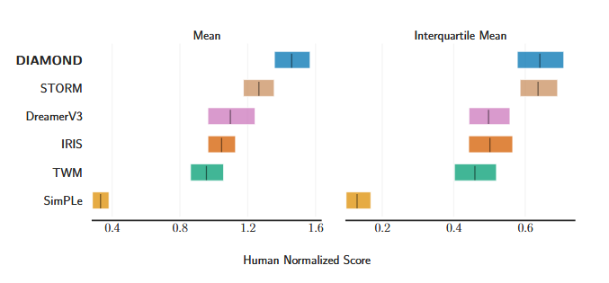
Figure 4: Mean and interquartile mean human normalized scores. Credit to (Alonso et al., 2024).

A key comparison is with IRIS, a world model based on a Variational Autoencoder (VAE) architecture. While IRIS generates plausible trajectories, they often suffer from visual inconsistencies between consecutive frames—for example, enemies being rendered as rewards or vice versa. Although these discrepancies may only affect a few pixels, they can drastically alter the agent’s learning process, as reward-related information is critical for policy optimization. In contrast, DIAMOND’s diffusion-based approach produces visually consistent trajectories, more accurately reflecting the true environment. These improvements in visual fidelity directly translate to stronger agent performance across several games.

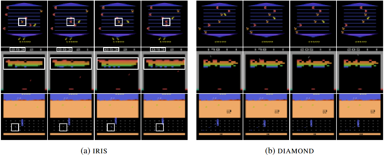
Figure 5: Consecutive frames imagined with IRIS (left) and DIAMOND (right). The white square highlights the visual inconsistencies. Credit to (Alonso et al., 2024).

Overall, DIAMOND provides compelling evidence that diffusion models can significantly advance world modeling for reinforcement learning, enabling more accurate, visually coherent, and data-efficient policy learning.

Limitations

While diffusion models offer promising capabilities for generative world modeling, several limitations remain when applying them within reinforcement learning (RL) settings:

• Discrete vs. Continuous Control: Current implementations are primarily evaluated in discrete action spaces. It remains uncertain how well these methods would generalize to continuous control environments, such as those involving robotic joint torques or accelerations.

• Limited Temporal Context: For computational efficiency, frame stacking is usually necessary. Instead of providing all past observations, the model only receives the last 𝐻 frames, introducing a form of short-term memory. However, this context is limited—information beyond 𝐻 steps is discarded. In scenarios with repetitive frames (e.g., static visual inputs like walls), the model may lose context and generate unrealistic or inconsistent dynamics.

• Reward and Termination Extraction: When integrating diffusion models into RL pipelines, it is not straightforward how to derive reward signals or termination conditions directly from the generative representation. For example, in the DIAMOND framework, a separate reward and termination model is used alongside the diffusion model to handle these aspects effectively.

References

Alonso, E., Jelley, A., Micheli, V., Kanervisto, A., Storkey, A., Pearce, T., et al. (2024). Diffusion for World Modeling: Visual Details Matter in Atari. Thirty-eighth Conference on Neural Information Processing Systems. https://arxiv.org/abs/2405.12399

Goodfellow, I. J., Pouget-Abadie, J., Mirza, M., Xu, B., Warde-Farley, D., Ozair, S., et al. (2014). Generative Adversarial Nets. Neural Information Processing Systems. https://api.semanticscholar.org/CorpusID:261560300

Ha, D. R., & Jü (2018). World Models. ArXiv, abs/1803.10122. https://api.semanticscholar.org/CorpusID:4807711

Hafner, D., Pasukonis, J., Ba, J., Lillicrap, T., & Lillicrap, T. (2023). Mastering Diverse Domains through World Models. ArXiv, abs/2301.04104. https://arxiv.org/abs/2301.04104

Kaiser, L., Babaeizadeh, M., Milos, P., Osinski, B., Campbell, R. H., Czechowski, K., et al. (2019). Model-Based Reinforcement Learning for Atari. International Conference on Learning Representations. https://arxiv.org/abs/1903.00374

Karras, T., Aittala, M., Aila, T., Laine, S., & Laine, S. (2022). Elucidating the Design Space of Diffusion-Based Generative Models. ArXiv, abs/2206.00364. https://api.semanticscholar.org/CorpusID:249240415

Kingma, D. P., & Welling, M. (2013). Auto-Encoding Variational Bayes. CoRR, abs/1312.6114. https://api.semanticscholar.org/CorpusID:216078090

Martí (2017). Towards Principled Methods for Training Generative Adversarial Networks. ArXiv, abs/1701.04862. https://api.semanticscholar.org/CorpusID:18828233

Micheli, V., Alonso, E., & Fleuret, F. (2023). Transformers are Sample-Efficient World Models. International Conference on Learning Representations. https://arxiv.org/abs/2209.00588

Rezende, D. J., & Mohamed, S. (2015). Variational Inference with Normalizing Flows. ArXiv, abs/1505.05770. https://api.semanticscholar.org/CorpusID:12554042

Robine, J., Höftmann, M., Uelwer, T., Harmeling, S., & Harmeling, S. (2023). Transformer-based World Models Are Happy With 100k Interactions. ArXiv, abs/2303.07109. https://arxiv.org/abs/2303.07109

Schrittwieser, J., Antonoglou, I., Hubert, T., Simonyan, K., Sifre, L., Schmitt, S., et al. (2019). Mastering Atari, Go, chess and shogi by planning with a learned model. Nature, 588, 604 - 609. https://api.semanticscholar.org/CorpusID:208158225

Sohl-Dickstein, J. N., Weiss, E. A., Maheswaranathan, N., Ganguli, S., & Ganguli, S. (2015). Deep Unsupervised Learning using Nonequilibrium Thermodynamics. ArXiv, abs/1503.03585. https://api.semanticscholar.org/CorpusID:14888175

Zhang, W., Wang, G., Sun, J., Yuan, Y., Huang, G., & Huang, G. (2023). STORM: Efficient Stochastic Transformer based World Models for Reinforcement Learning. Advances in Neural Information Processing Systems, 36. https://arxiv.org/abs/2310.09615

McCloud, S. (1993). Understanding Comics: The Invisible Art. Tundra Publishing. https://en.wikipedia.org/wiki/Understanding_Comics